Shashi Tharoor: Why nations should pursue "soft" power | Video on TED.com

Shashi Tharoor: Why nations should pursue "soft" power | Video on TED.com

LPS-ATE: produce terrain withoutfloating points

Problem:
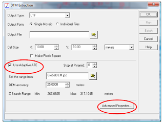
When using LPS-ATE without changing any of the parameters, the “Use Adaptive ATE” setting is turned on. Also the smoothing option in the default strategy parameter is set to low smoothing. This setting could result in calculatedterrain points floating above the ground (In some cases more than 50% of the total results.). Often LPS users justtake the default settings when making a first run in LPS ATE for a terrain.
Recommendation: Use the no smoothing option when the “Use Adaptive ATE” is switched on.

Solution:
When defining the settings for your DEM, use “Adaptive ATE.”(Picture1)

In the advanced properties, select the Area Selection tab.(Picture2)


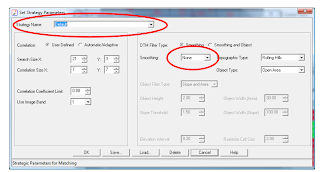
Select Strategy Parameters in (Picture 3) Use the settings for default and set the smoothing parameters to NONE!!
With these settings, the problem with floating points above the ground after ATE is solved and most of thepoints (80 - 90%) are on the ground.

Picture (1):

Picture(2):

Picture(3):

Job Opportunities in Nationalized Banks

SBI

UBI

UCO BANK

UNITED BANK OF INDIA

CENTRAL BANK OF INDIA

CANARA BANK

BANK OF BARODA

RESERVE BANK OF INDIA

NABARD

INDIAN OVERSEAS BANK

ALLAHABAD BANK

PUBJAB NATIONAL BANK

Topographical Maps of the World

Topogrophical Maps to India, Pakistan, Bangladesh and Srilanka

North Africa

Europe

ERDAS LPS

Creating Orthorectified Aerial Photography Without A Camera Calibration

Introduction

To make precisely orthorectified aerial photographs using IMAGINE OrthoBASE, generally you need the camera calibration report to identify the interior parameters such as focal length, principal points and fiducial marks of the frame camera used to capture your photography. However, there are times when you may not be able to get the report. Even in such cases, some of the parameters can be derived from your photography and used in your ortho-rectification process.

Of course, the non-metric model or digital camera model that doesn’t need fiducial marks are also useful in this case, but using the frame camera model and
estimating the interior orientation information will give more accurate results.
Input Data
• Aerial photography
• Ground control points (GCPs) with x, y, z coordinates
• DEMs
* Assumption: Camera calibration report is not available

How to Get Camera Information?

To define the frame camera model, we have to input, at a minimum, the following three kinds of information – principal point, focal length and the coordinates of the fiducial marks. In case you don’t have the camera calibration report, you need to get these parameters from somewhere else. This information can be derived from your photography.

1. Principal Point

The principal point is mathematically defined as the intersection of the
perpendicular line through the perspective center of the image plane. If the optical system
of camera has some distortion, this point will be slightly different from the center of
photography. Thinking inversely, this point corresponds to the center of photography
when an ideal camera is assumed. Under this assumption, you can use value x, y = 0, 0 as
the principal point coordinate.

2. Focal Length

In typical aerial photography, you can find the value of the focal length captured
in the data strip. Below is an example of NAPP (National Aerial Photography Program)
photography captured by a Wild camera. The focal length can be identified as 152.81mm.

3. Fiducial Marks

The coordinates of fiducial marks can be measured directly using a ruler on the
hardcopy photography. Take the origin of coordinates at the point where the diagonal
lines connecting fiducial marks meet. At least four fiducial marks must be measured in
millimeter units.

The coordinate system should be defined according to the location of the data
strip, i.e., you should take the Y-axis in the direction along which the data strip lies. The
order of marks is typically defined as shown in following diagram.
w
#1 Data Strip #3
PP Y
h
(0, 0)
X
#4 #2
Once you have measured the distance between fiducial marks both horizontally
(w) and vertically (h), the coordinates are easily defined, as in the following table
according to the origin and orientation of coordinate system mentioned above.

X Y
#1 - h/2 - w/2
#2 h/2 w/2
#3 - h/2 w/2
#4 h/2 - w/2
Table 1. Coordinate values of fiducial marks (Units; mm)
If you have digitized photography but know in what resolution it was scanned,
you can measure the length with the Measurement Tool of the IMAGINE Viewer and
divide it by the scanning resolution. For example, if the scanning resolution is 300 dpi
(dots per inch) and the length (w) measured in the Viewer is 2500 pixels, the mm length
can be easily calculated as,
w = (2500 / 300) × 25.4 = 211.67 mm.
In case your photography doesn’t have the focal length information captured, if
you do know the flight height (H) and photo scale (1/S), you can calculate the rough
value from the following simple expression. Of course, the flight height must be
converted to meter units.
Focal length ≈ H / S
You may also find a rough value from photogrammetry manuals if you have
information on what model of camera was used for the photography.
Self-calibrating Bundle Adjustment (SCBA) IMAGINE OrthoBASE can automatically correct these rough camera parameters in the triangulation process by the method called SCBA. Accuracy should be reasonably sufficient with the focal length in the data strip. But for those applications where greater accuracy is required or only rough focal length is available, SCBA may be worthwhile. It is advisable to obtain a reasonable RMSE without SCBA first prior to selecting to use an SCBA because it requires more GCPs than usual due to the additional unknowns of the
focal length, etc. Also, it is recommended to use only two to three images in order to find
the adjusted focal length before applying it to a whole block of more images.

IMAGINE OrthoBASE Workflow

The following steps can be used to orthorectify aerial photography without a calibration
report. In this case, we ortho-rectify using the following data, which are included in the
“examples” directory of ERDAS IMAGINE.
• Aerial Photograph (Input Data): ps_napp.img
• DEM: ps_dem.img
• GCPs: ps_camera.gcc
NOTE: Although we process only one photograph in this example, this method also can
be applied to multiple images.
Step 1. Define the IMAGINE OrthoBASE Block File
Input the following information to define the IMAGINE OrthoBASE project:
• The IMAGINE OrthoBASE Block file name. The block file is a binary file that
contains all of the information associated with a project. This includes the number
of images processed, GCPs used, image coordinate information, projection, units,
etc.
• Select the Frame Camera geometric model.
• Projection, spheroid and datum should be same as DEM and GCPs. In this case,
- Projection: UTM Zone 11
- Spheroid: Clarke 1866
- Datum: NAD27
• Horizontal, vertical and angular units are Meter, Meter and Degree.
• Type of rotation used to define the orientation of the camera as it existed at the
time of exposure. In this case, the Omega, Phi and Kappa rotation systems are
used.
• Type of photography/imagery used (including aerial or terrestrial). If aerial
photography/imagery is used, the photographic direction is the Z-Axis. In this
case, the Z-Axis option is selected.
• Average flying height of the camera. The average flying height of the aircraft is
not required for this case.

Step 2. Add imagery to the project

To add images to the block, select the Add Images icon or Edit | Add
Frame... option from menu. Within the Image File Name chooser, identify and select the
image to be added. In this case, select ps_napp.img from examples directory.

Step 3. Create Pyramid Layers

Once the images have been input and defined, the pyramid layers associated with
the image can be created. Selecting one of the red cell elements contained within the Pyr
column will open the Compute Pyramid Layers dialog.

Selecting the All Images Without Pyramids option will consecutively create
pyramid layers for each image in the block project. Once the pyramid layers have been
created, the Pyr cell elements will change to green. The pyramid layers optimize image
handling during display, as well as the performance of automatic tie point collection.

Step 4. Input camera parameters

Start the Frame Editor by selecting the Show and Edit Frame Properties icon
or Edit | Frame Editor... Then press the New... button in the Sensor tab. You may
then input camera parameters we discussed above.

4-1. General Tab

You can input Focal Length and Principal Point here. With regard to the focal
length, you can find the value at the top of the ps_napp.img. (Open the file in a Viewer
and check it.)

4-2. Fiducials Tab

Here, you can input fiducial coordinates that are summarized in Table 1. Set the
Number of Fiducials to the same number as the fiducial marks on your photography, in
this case 4, and type the coordinate values you measured in the Film X and Film Y
columns.

You can save these parameters with the Save button. Pressing OK will apply this
setting and close the dialog. By defining the camera within the Camera Information
dialog, the information will be applied to each image in the block project.

4-3. Fiducial Measurement Click the Interior Orientation Tab of the Frame Editor. You can see the fiducial
mark coordinates in the CellArray. The fiducial mark positions on the image coordinate
system can be measured within this dialog. Clicking the Open viewer for image fiducial
will show three embedded viewers in which you can select the
measurement icon point with mouse cursor. Before selecting the point, make sure that you are selecting
appropriate Fiducial Orientations.
In this example, you should select icon because the Y-axis of ps_napp.img
can be identified as right from the location of the data strip of the photograph.

When all of Fiducials are measured, click OK button and close this dialog.

Step 5. GCP Collection

In this step, we define ground control points (GCPs). Since we process only one
image in this example, we should collect as many GCPs as possible. There is a GCP file
named ps_camera.gcc in the examples directory that can be used.
will open a window that Selecting the Start point measurement tool icon
has three embedded viewers. First, load the GCP file ps_camera.gcc with the Reset
horizontal reference source icon.
Second, enter the file coordinates in the right CellArray. Coordinates
corresponding to each reference coordinates are shown in following table. Notice that
you have to create a row in the table (and a point) by clicking somewhere you like in the

viewer using Create Point tool before enter file coordinates. Once a row is created, you
can enter the correct coordinate values into the column X File and Y File. The point will
automatically move to the correct position.
No. X File Y File X Reference Y Reference
1 1401.178 2101.549716 544657.8972 3740719.772
2 850.1665 2214.532185 542301.2512 3740224.479
3 808.0213 571.7258523 541989.3150 3747260.594
4 1270.101 1271.887784 544030.3503 3744286.400
5 1687.295 590.5027834 545787.2657 3747269.691
6 2146.066 2223.599887 547900.7802 3740212.455
7 2019.663 1107.192155 547285.4195 3745049.591
8 150.7457 630.5894886 539235.5851 3746921.105
9 165.4252 1525.152586 539516.8989 3743200.150
10 163.5571 2181.081535 539801.9035 3740804.110
Table 2. File and Reference Coordinates of GCPs (ps_camera.gcc)
[4] The point
[2] Make a
automatically
point by
moves to the
clicking
correct position
anywhere you
like
[3] Enter the
correct File
Coordinate here
[1] Select
a row
NOTE: Before going to next step, select GCP and click Active column and make it
inactive (dismiss X mark) because it’s a bad GCP.

Step 6. Perform Block Triangulation

Click the Triangulation Property icon on the Point Measurement Tool and
edit Triangulation Property. Open the Point tab and set the Type field to Same weighted
values.

In case you are using rough focal length, self-calibration capability will correct
this automatically while following the triangulation process. It is available if you select
Same unweighted correction for all in the Interior tab.

Selecting the Run button will execute triangulation. The resulting accuracy of the
triangulation can be checked in the Triangulation Summary dialog or report. Then press
Update button to reflect the triangulation results to Exterior Orientation Parameters.
(You can see this in the Frame Editor.) Close the Triangulation Summary and Point
Measurement Tool and go to next step.

Step 7. Rectify the Images

Selecting the Start ortho resampling process icon will display the Ortho
Resampling dialog. Set the output file name as you like and select ps_dem.img as the

DEM. Output Cell Size, Output Extent and Resampling Method, etc., also can be specified here.

Step 8. Check the result

Open the output file on the Viewer and overlay other GIS data.